Week 6 - More about pandas

import pandas as pd
import numpy as np
import matplotlib.pyplot as plt
%matplotlib inline
plt.style.use('bmh')

We’ve looked at Series, DataFrame, how to view, select and index data, and how to make plots with pandas. Now we will look at time series data, which pandas is simply brilliant for working with.

‘Time series data’ refers to any form of data that is represented or indexed with ordered timestamps. Examples include stock prices, electrical activity in the brain, and temperature throughout the day. As you might have guessed, this involves dates, times, and differences between them.

Timestamp and Timedelta

In pandas, dates and times are represented with pd.Timestamp, which is a replacement for Python’s native datetime.datetime object. The two are interchangeable in many respects, but a key difference is that pd.Timestamp uses NumPy’s datetime64 and timedelta64 data types and incorporates a much wider range of functionality and powerful features for creating and manipulating time series.

---

• pd.Timestamp - Read more here

• datetime.datetime - Read more here

• datetime64 and timedelta64 - Read more here

---

Let’s create timestamps to mark two memorable points in history. The First World War ended in 1918 at the eleventh hour of the eleventh day of the eleventh month, and the Second World War ended on the 08 May at one-minute past 11 in the evening.

end_of_ww1 = pd.Timestamp('1918-11-11 11:00:00')  # Armistice Day
end_of_ww2 = pd.Timestamp('1945-05-08 23:01:00')  # VE Day

Timestamp data have many useful methods. An especially useful method is .strftime(), which creates a str representation of a timestamp using various formatting codes. Here are some examples.

print("The First World War ended", end_of_ww1.strftime('%d %B %Y'), "at", end_of_ww1.strftime('%I:%M %p'))
print("The Second World War ended", end_of_ww2.strftime('%d %B %Y'), "at", end_of_ww2.strftime('%I:%M %p'))

The First World War ended 11 November 1918 at 11:00 AM
The Second World War ended 08 May 1945 at 11:01 PM

Here, the % symbols and subsequent characters tell the strftime() method how to represent the timestamp. You may wish to experiment with other formatting codes to format the timestamps in different ways. Copy the above code into the cell below and try to format the dates using abbreviated month names and 24-hour time.

If you are a history buff, you may already know the day of the week when each of The Great Wars ended. If not, you can find out using the pd.Timestamp.day_name() method.

print('The First World War ended on a', end_of_ww1.day_name())
print('The Second World War ended on a', end_of_ww2.day_name())

The First World War ended on a Monday
The Second World War ended on a Tuesday

If we have two timestamps, we can calculate the difference between them, which is known as a Timedelta. Let’s do this to find out how much time elapsed between the end of the First and Second World Wars.

tdelta = end_of_ww2 - end_of_ww1  # Subtract the end of WW1 from the end of WW2
print('Time between the end of the First and Second World Wars:')
print(f'{tdelta.days} days and {tdelta.seconds} seconds')

Time between the end of the First and Second World Wars:
9675 days and 43260 seconds

A Timedelta behaves like a number in many respects and can be operated on with most mathematical operators. But there are restrictions. For example, one can divide or multiply a Timedelta by any number, but addition and subtraction can only take place with other Timestamp or Timedelta objects. If you think about it, this makes perfect sense.

print('Time between end of WW1 and WW2: ', tdelta)
print('Multiplied by 3:                 ', tdelta * 3)
print('Divided by 2:                    ', tdelta / 2)
print('Added to itself:                 ', tdelta + tdelta)
print('Minus twice itself:              ', tdelta - (tdelta * 2))

Time between end of WW1 and WW2:  9675 days 12:01:00
Multiplied by 3:                  29026 days 12:03:00
Divided by 2:                     4837 days 18:00:30
Added to itself:                  19351 days 00:02:00
Minus twice itself:               -9676 days +11:59:00

If you try to perform an operation that is not supported, such as raising a Timedelta to some power or multiplying two Timedelta’s together, you will get an error.

tdelta ** 2  # Can not raise a Timedelta to a power...

---------------------------------------------------------------------------
TypeError                                 Traceback (most recent call last)
/var/folders/c9/7yddvl1n2ss863cgfngj0wpm0000gp/T/ipykernel_41875/977053077.py in <module>
----> 1 tdelta ** 2  # Can not raise a Timedelta to a power...

TypeError: unsupported operand type(s) for ** or pow(): 'Timedelta' and 'int'

In case you are wondering, leap years and other time-related idiosyncrasies are dealt with implicitly.

leap_year = pd.Timestamp('27 Feb 2020')  # 2020 was a leap year
print((leap_year + pd.Timedelta('2D')).strftime('%d %B %Y'))  # Add 2 days

29 February 2020

not_a_leap_year = pd.Timestamp('27 Feb 2021')  # 2021 wasn't a leap year
print((not_a_leap_year + pd.Timedelta('2D')).strftime('%d %B %Y'))  # Add 2 days

01 March 2021

Working with dates and times

Previously we have encountered functions such as range() and np.linspace(), which produce sequences of evenly-spaced numeric data. In pandas, we can do the same with dates using the pd.date_range(...) function. Let’s use it to create a timestamp for every day of this year.

ts = pd.date_range(start='2022-01-01', end='2022-12-31', freq='D', inclusive='both')
ts

DatetimeIndex(['2022-01-01', '2022-01-02', '2022-01-03', '2022-01-04',
               '2022-01-05', '2022-01-06', '2022-01-07', '2022-01-08',
               '2022-01-09', '2022-01-10',
               ...
               '2022-12-22', '2022-12-23', '2022-12-24', '2022-12-25',
               '2022-12-26', '2022-12-27', '2022-12-28', '2022-12-29',
               '2022-12-30', '2022-12-31'],
              dtype='datetime64[ns]', length=365, freq='D')

The result is a DatetimeIndex, which may be used as the index for a Series or DataFrame. Let’s work some magic on these timestamps to get a list of all future dates for this year in long-format.

# Get all future dates for this year and format them nicely
ts[ts > pd.Timestamp.now()].strftime('%A %d %B %Y').tolist()

['Wednesday 21 December 2022',
 'Thursday 22 December 2022',
 'Friday 23 December 2022',
 'Saturday 24 December 2022',
 'Sunday 25 December 2022',
 'Monday 26 December 2022',
 'Tuesday 27 December 2022',
 'Wednesday 28 December 2022',
 'Thursday 29 December 2022',
 'Friday 30 December 2022',
 'Saturday 31 December 2022']

As you can see, a DatetimeIndex is a powerful and flexible tool for representing dates and times. When it really starts to shine is when it is used as the index for time series data, so let’s invent some.

Imagine there is a shop that opened at the turn of the millennium which sells apples, bananas and cakes. At the time of opening, these items were sold at the respective prices of £0.45, £0.28, and £0.62 per item, but there’s been some inflation over time. Each day, a random(ish) number of each item is sold. Cakes are most popular, then bananas, then apples.

# Initial cost in year 2000
cost_of_apple = 0.45
cost_of_banana = 0.28
cost_of_cake = 0.62

# Create a range of dates from 2000 to 2022 with 1-day frequency.
# This means we will have a row for every day.
dates = pd.date_range('2000', '2022', freq='1D')
number_of_days = len(dates)

# Create the DataFrame
df = pd.DataFrame(
    {
        'date': dates,
        'apples_sold': np.random.randint(0, 200, number_of_days),
        'bananas_sold': np.random.randint(0, 350, number_of_days),
        'cakes_sold': np.random.randint(0, 700, number_of_days),
        'cost_of_apple' : cost_of_apple,
        'cost_of_banana': cost_of_banana,
        'cost_of_cake': cost_of_cake
    },
)

# Adjust costs for inflation
cost_cols = ['cost_of_apple', 'cost_of_banana', 'cost_of_cake']
inflation = np.exp(np.linspace(0, 1, number_of_days))
df[cost_cols] = df[cost_cols].mul(inflation, axis=0)

# New columns for profit
df['apples_profit'] = df['apples_sold'] * df['cost_of_apple']
df['bananas_profit'] = df['bananas_sold'] * df['cost_of_banana']
df['cakes_profit'] = df['cakes_sold'] * df['cost_of_cake']
df['total_profit'] = df.apples_profit + df.bananas_profit + df.cakes_profit
df = df.round(2)
df

	date	apples_sold	bananas_sold	cakes_sold	cost_of_apple	cost_of_banana	cost_of_cake	apples_profit	bananas_profit	cakes_profit	total_profit
0	2000-01-01	199	347	539	0.45	0.28	0.62	89.55	97.16	334.18	520.89
1	2000-01-02	179	19	693	0.45	0.28	0.62	80.56	5.32	429.71	515.59
2	2000-01-03	178	215	447	0.45	0.28	0.62	80.12	60.21	277.21	417.54
3	2000-01-04	22	165	578	0.45	0.28	0.62	9.90	46.22	358.49	414.61
4	2000-01-05	23	1	294	0.45	0.28	0.62	10.36	0.28	182.37	193.01
...	...	...	...	...	...	...	...	...	...	...	...
8032	2021-12-28	157	6	411	1.22	0.76	1.68	191.95	4.56	692.33	888.84
8033	2021-12-29	1	255	106	1.22	0.76	1.68	1.22	194.01	178.58	373.81
8034	2021-12-30	71	326	545	1.22	0.76	1.68	86.83	248.06	918.28	1253.17
8035	2021-12-31	106	36	617	1.22	0.76	1.69	129.65	27.40	1039.72	1196.76
8036	2022-01-01	167	169	40	1.22	0.76	1.69	204.28	128.63	67.41	400.32

8037 rows × 11 columns

Now, if we look at the data types of the DataFrame, we can see that the date column has type datetime64[ns].

df.dtypes

date              datetime64[ns]
apples_sold                int64
bananas_sold               int64
cakes_sold                 int64
cost_of_apple            float64
cost_of_banana           float64
cost_of_cake             float64
apples_profit            float64
bananas_profit           float64
cakes_profit             float64
total_profit             float64
dtype: object

When working with the world population and titanic datasets, we used the str accessor method to interface with additional string methods (e.g., df['name'].str.contains('Smith')). For datetime-like data, there is a dt accessor method, which opens the door to datetime functionality. Below, we use the dt accessor method to create a separate column containing the day of the week, the year, and the fiscal year.

df['Day'] = df['date'].dt.day_name()  # Get day of week
df['Year'] = df['date'].dt.year  # Get current year
df['Fiscal Year'] = df['date'].dt.to_period('Q-APR').dt.qyear  # Get fiscal year
df.tail()

	date	apples_sold	bananas_sold	cakes_sold	cost_of_apple	cost_of_banana	cost_of_cake	apples_profit	bananas_profit	cakes_profit	total_profit	Day	Year	Fiscal Year
8032	2021-12-28	157	6	411	1.22	0.76	1.68	191.95	4.56	692.33	888.84	Tuesday	2021	2022
8033	2021-12-29	1	255	106	1.22	0.76	1.68	1.22	194.01	178.58	373.81	Wednesday	2021	2022
8034	2021-12-30	71	326	545	1.22	0.76	1.68	86.83	248.06	918.28	1253.17	Thursday	2021	2022
8035	2021-12-31	106	36	617	1.22	0.76	1.69	129.65	27.40	1039.72	1196.76	Friday	2021	2022
8036	2022-01-01	167	169	40	1.22	0.76	1.69	204.28	128.63	67.41	400.32	Saturday	2022	2022

We now have three new and useful columns in our DataFrame. At the moment, the original date column is just a column of data, but what we really need is for it to be our index.

# Set the date column as the index
df = df.set_index('date')
df

	apples_sold	bananas_sold	cakes_sold	cost_of_apple	cost_of_banana	cost_of_cake	apples_profit	bananas_profit	cakes_profit	total_profit	Day	Year	Fiscal Year
date
2000-01-01	199	347	539	0.45	0.28	0.62	89.55	97.16	334.18	520.89	Saturday	2000	2000
2000-01-02	179	19	693	0.45	0.28	0.62	80.56	5.32	429.71	515.59	Sunday	2000	2000
2000-01-03	178	215	447	0.45	0.28	0.62	80.12	60.21	277.21	417.54	Monday	2000	2000
2000-01-04	22	165	578	0.45	0.28	0.62	9.90	46.22	358.49	414.61	Tuesday	2000	2000
2000-01-05	23	1	294	0.45	0.28	0.62	10.36	0.28	182.37	193.01	Wednesday	2000	2000
...	...	...	...	...	...	...	...	...	...	...	...	...	...
2021-12-28	157	6	411	1.22	0.76	1.68	191.95	4.56	692.33	888.84	Tuesday	2021	2022
2021-12-29	1	255	106	1.22	0.76	1.68	1.22	194.01	178.58	373.81	Wednesday	2021	2022
2021-12-30	71	326	545	1.22	0.76	1.68	86.83	248.06	918.28	1253.17	Thursday	2021	2022
2021-12-31	106	36	617	1.22	0.76	1.69	129.65	27.40	1039.72	1196.76	Friday	2021	2022
2022-01-01	167	169	40	1.22	0.76	1.69	204.28	128.63	67.41	400.32	Saturday	2022	2022

8037 rows × 13 columns

Now we can index the DataFrame using any valid date/time string, of which there are many. For example, if we wanted to look at the information for a particular day, say, 23 April 2012, we could use any of the following:

• '2012-04-23'

• 'April 23, 2012'

• '23 Apr 2012'

• '23 April 2012'

• '2012/04/23'

df.loc['23 April 2012']  # St Georges day, 2012

apples_sold           54
bananas_sold         250
cakes_sold           605
cost_of_apple       0.79
cost_of_banana      0.49
cost_of_cake        1.08
apples_profit      42.52
bananas_profit    122.48
cakes_profit      656.34
total_profit      821.34
Day               Monday
Year                2012
Fiscal Year         2012
Name: 2012-04-23 00:00:00, dtype: object

Try experimenting with different indexing strings!

If you want the data for an entire year, just pass in the year.

df.loc['2012']  # Get all data from 2012

	apples_sold	bananas_sold	cakes_sold	cost_of_apple	cost_of_banana	cost_of_cake	apples_profit	bananas_profit	cakes_profit	total_profit	Day	Year	Fiscal Year
date
2012-01-01	68	166	389	0.78	0.48	1.07	52.80	80.19	416.12	549.10	Sunday	2012	2012
2012-01-02	77	238	240	0.78	0.48	1.07	59.79	114.99	256.76	431.54	Monday	2012	2012
2012-01-03	37	319	98	0.78	0.48	1.07	28.73	154.15	104.86	287.74	Tuesday	2012	2012
2012-01-04	133	173	8	0.78	0.48	1.07	103.30	83.61	8.56	195.47	Wednesday	2012	2012
2012-01-05	128	316	339	0.78	0.48	1.07	99.43	152.73	362.81	614.97	Thursday	2012	2012
...	...	...	...	...	...	...	...	...	...	...	...	...	...
2012-12-27	158	144	552	0.81	0.51	1.12	128.31	72.76	617.61	818.68	Thursday	2012	2013
2012-12-28	167	75	72	0.81	0.51	1.12	135.63	37.90	80.57	254.10	Friday	2012	2013
2012-12-29	41	1	11	0.81	0.51	1.12	33.30	0.51	12.31	46.12	Saturday	2012	2013
2012-12-30	152	277	680	0.81	0.51	1.12	123.48	140.02	761.11	1024.61	Sunday	2012	2013
2012-12-31	78	255	45	0.81	0.51	1.12	63.37	128.91	50.37	242.66	Monday	2012	2013

366 rows × 13 columns

Looks like 2012 was a leap year, because there are 366 days. Let’s check this by getting the data for February of that year. To do this, we just need to add the month.

df.loc['2012-02']  # February 2012

	apples_sold	bananas_sold	cakes_sold	cost_of_apple	cost_of_banana	cost_of_cake	apples_profit	bananas_profit	cakes_profit	total_profit	Day	Year	Fiscal Year
date
2012-02-01	198	309	540	0.78	0.48	1.07	154.32	149.85	579.87	884.05	Wednesday	2012	2012
2012-02-02	130	140	48	0.78	0.49	1.07	101.33	67.90	51.55	220.79	Thursday	2012	2012
2012-02-03	83	164	500	0.78	0.49	1.07	64.71	79.55	537.05	681.31	Friday	2012	2012
2012-02-04	34	221	292	0.78	0.49	1.07	26.51	107.22	313.68	447.40	Saturday	2012	2012
2012-02-05	130	18	180	0.78	0.49	1.07	101.37	8.73	193.39	303.49	Sunday	2012	2012
2012-02-06	113	126	361	0.78	0.49	1.07	88.13	61.14	387.90	537.17	Monday	2012	2012
2012-02-07	77	337	92	0.78	0.49	1.07	60.06	163.55	98.87	322.48	Tuesday	2012	2012
2012-02-08	156	343	576	0.78	0.49	1.07	121.69	166.49	619.07	907.25	Wednesday	2012	2012
2012-02-09	101	194	116	0.78	0.49	1.07	78.80	94.18	124.69	297.66	Thursday	2012	2012
2012-02-10	65	234	179	0.78	0.49	1.08	50.72	113.61	192.43	356.76	Friday	2012	2012
2012-02-11	60	248	446	0.78	0.49	1.08	46.82	120.42	479.53	646.77	Saturday	2012	2012
2012-02-12	167	31	444	0.78	0.49	1.08	130.34	15.05	477.44	622.83	Sunday	2012	2012
2012-02-13	131	64	32	0.78	0.49	1.08	102.25	31.08	34.41	167.75	Monday	2012	2012
2012-02-14	144	232	244	0.78	0.49	1.08	112.42	112.69	262.44	487.55	Tuesday	2012	2012
2012-02-15	174	232	603	0.78	0.49	1.08	135.85	112.71	648.66	897.21	Wednesday	2012	2012
2012-02-16	100	25	503	0.78	0.49	1.08	78.09	12.15	541.15	631.38	Thursday	2012	2012
2012-02-17	4	133	649	0.78	0.49	1.08	3.12	64.63	698.31	766.06	Friday	2012	2012
2012-02-18	95	71	357	0.78	0.49	1.08	74.20	34.51	384.17	492.88	Saturday	2012	2012
2012-02-19	134	224	518	0.78	0.49	1.08	104.67	108.87	557.50	771.05	Sunday	2012	2012
2012-02-20	10	337	170	0.78	0.49	1.08	7.81	163.82	182.99	354.62	Monday	2012	2012
2012-02-21	85	63	388	0.78	0.49	1.08	66.41	30.63	417.69	514.73	Tuesday	2012	2012
2012-02-22	190	284	312	0.78	0.49	1.08	148.47	138.09	335.92	622.48	Wednesday	2012	2012
2012-02-23	190	18	562	0.78	0.49	1.08	148.49	8.75	605.15	762.40	Thursday	2012	2012
2012-02-24	96	246	331	0.78	0.49	1.08	75.04	119.64	356.46	551.14	Friday	2012	2012
2012-02-25	4	151	333	0.78	0.49	1.08	3.13	73.45	358.66	435.23	Saturday	2012	2012
2012-02-26	118	176	388	0.78	0.49	1.08	92.26	85.62	417.95	595.82	Sunday	2012	2012
2012-02-27	111	337	277	0.78	0.49	1.08	86.79	163.96	298.42	549.17	Monday	2012	2012
2012-02-28	60	257	163	0.78	0.49	1.08	46.92	125.05	175.63	347.60	Tuesday	2012	2012
2012-02-29	197	309	288	0.78	0.49	1.08	154.08	150.38	310.35	614.80	Wednesday	2012	2012

We can also ‘slice’ a DataFrame with a DatetimeIndex using date strings. Let’s grab the data for the last four days of August 2014.

df.loc['2014-08-28':'2014-08-31']  # Last 4 days of August 2014

	apples_sold	bananas_sold	cakes_sold	cost_of_apple	cost_of_banana	cost_of_cake	apples_profit	bananas_profit	cakes_profit	total_profit	Day	Year	Fiscal Year
date
2014-08-28	125	63	266	0.88	0.55	1.21	109.50	34.34	321.05	464.89	Thursday	2014	2015
2014-08-29	77	135	450	0.88	0.55	1.21	67.46	73.59	543.19	684.25	Friday	2014	2015
2014-08-30	8	122	435	0.88	0.55	1.21	7.01	66.52	525.15	598.68	Saturday	2014	2015
2014-08-31	124	8	467	0.88	0.55	1.21	108.67	4.36	563.85	676.88	Sunday	2014	2015

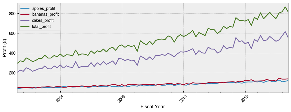
To round things off, let’s group the data by quarters of the fiscal year (which starts in April) and plot mean profit over time.

# A new column for quarters of the fiscal year
df['Fiscal Year'] = df.index.to_period('Q-APR')
df.head()

	apples_sold	bananas_sold	cakes_sold	cost_of_apple	cost_of_banana	cost_of_cake	apples_profit	bananas_profit	cakes_profit	total_profit	Day	Year	Fiscal Year
date
2000-01-01	199	347	539	0.45	0.28	0.62	89.55	97.16	334.18	520.89	Saturday	2000	2000Q3
2000-01-02	179	19	693	0.45	0.28	0.62	80.56	5.32	429.71	515.59	Sunday	2000	2000Q3
2000-01-03	178	215	447	0.45	0.28	0.62	80.12	60.21	277.21	417.54	Monday	2000	2000Q3
2000-01-04	22	165	578	0.45	0.28	0.62	9.90	46.22	358.49	414.61	Tuesday	2000	2000Q3
2000-01-05	23	1	294	0.45	0.28	0.62	10.36	0.28	182.37	193.01	Wednesday	2000	2000Q3

# Get the profit columns
profit_cols = df.columns[df.columns.str.endswith('profit')]
(
    df.groupby('Fiscal Year')[profit_cols]
    .mean()
    .plot(ylabel='Profit (£)', figsize=(12, 4), rot=45)
);

If you can master tricks like this in pandas, the world of time series data is at your fingertips.

---

• pandas - Follow this link to learn more about Time Series / Date functionality

---