Week 6 - Exercises

Exercise 1 - GB cycling accidents

In the data folder of the course materials you should find a CSV file called gb_cycling_accidents.csv which contains data on bicycle accidents in Great Britain from 1970 to 2018. I retrieved the data set from kaggle, which cites data.world as the original source. Each row holds information about a specific accident, and each column holds information about the accident, such as the date, time of day, day of week, number of vehicles involved, weather conditions, severity, etc. Here is the full explanation of the columns in the data set.

Variable	Definition
Accident_Index	Unique identifier for the accident. This may be thought of as the accident “case number”.
Number_of_Vehicles	Number of vehicles that were involved in the accident
Number_of_Casualties	Number of casualties resulting from the accident
Date	Date when the accident happened
Time	Time when the accident happened
Speed_limit	Speed limit on the part of the road where the accident took place
Road_conditions	Road condition (e.g., “frost”) at the time and place of the accident
Weather_conditions	Whether condition (e.g., “rain”) at time and place of the accident
Day	Day of the week when the accident occurred
Road_type	Type of road (e.g., “Dual carriageway”) where the accident happened
Light_conditions	Light conditions (e.g., “Daylight”) at time of accident
Gender	Whether the accident victim was Male or Female
Severity	How severe (e.g., “Serious”) the accident was
Age_Grp	Age group of the accident victim

Let’s explore the frequency of accidents with respect to the different variables.

import numpy as np
import matplotlib.pyplot as plt
%matplotlib inline
plt.style.use('bmh')

1. Import pandas and read data/gb_cycling_accidents.csv into a DataFrame

import pandas as pd

df = pd.read_csv('../data/gb_cycling_accidents.csv')
df

	Accident_Index	Number_of_Vehicles	Number_of_Casualties	Date	Time	Speed_limit	Road_conditions	Weather_conditions	Day	Road_type	Light_conditions	Gender	Severity	Age_Grp
0	197901A1SEE71	2	1	1979-01-01	18:20	50.0	Snow	Unknown	Monday	Dual carriageway	Darkness lights lit	Male	Serious	36 to 45
1	197901A2JDW40	1	1	1979-02-01	09:15	30.0	Snow	Unknown	Tuesday	Unknown	Daylight	Male	Slight	46 to 55
2	197901A4IJV90	2	1	1979-04-01	08:45	30.0	Snow	Unknown	Thursday	Unknown	Daylight	Male	Slight	46 to 55
3	197901A4NIE33	2	1	1979-04-01	13:40	30.0	Wet	Unknown	Thursday	Unknown	Daylight	Male	Slight	36 to 45
4	197901A4SKO47	2	1	1979-04-01	18:50	30.0	Wet	Unknown	Thursday	Unknown	Darkness lights lit	Male	Slight	46 to 55
...	...	...	...	...	...	...	...	...	...	...	...	...	...	...
827856	2018983118818	2	1	2018-02-07	14:55	30.0	Dry	Clear	Monday	Single carriageway	Daylight	Male	Slight	6 to 10
827857	2018983119218	2	1	2018-07-24	07:45	30.0	Dry	Clear	Tuesday	Single carriageway	Daylight	Male	Serious	56 to 65
827858	2018983120618	2	1	2018-10-08	13:25	20.0	Dry	Clear	Friday	Single carriageway	Daylight	Male	Serious	11 to 15
827859	2018983121918	2	1	2018-07-18	21:10	30.0	Dry	Clear	Wednesday	Single carriageway	Daylight	Male	Serious	46 to 55
827860	2018983133818	2	1	2018-12-20	15:14	30.0	Wet	Rain	Thursday	Single carriageway	Daylight	Male	Serious	6 to 10

827861 rows × 14 columns

2. How many unique values are in the following columns?

• Speed_limit

• Road_conditions

• Weather_conditions

• Road_type

• Light_conditions

• Gender

• Severity

• Age_Grp

cols = [
    'Speed_limit',
    'Road_conditions',
    'Weather_conditions',
    'Road_type',
    'Light_conditions',
    'Gender',
    'Severity',
    'Age_Grp'
]

for col in cols:
    print(f'{col}: {df[col].unique()}')  # Use .unique() to get the unique values

Speed_limit: [ 50.  30.  40.  70.  60.  38.  25.   0.  10.  15.  20.  36.  32.  33.
  34.  46.  66.  35.  31.  55.  51.  61.  41.  39.  21.  16.  22.  27.
  26.  13.  45.  59. 660.   5.   3.  62.]
Road_conditions: ['Snow' 'Wet' 'Dry' 'Frost' 'Flood' 'Missing Data']
Weather_conditions: ['Unknown' 'Rain' 'Snow' 'Fog' 'Clear' 'Clear and windy' 'Other'
 'Rain and windy' 'Snow and windy' 'Missing data']
Road_type: ['Dual carriageway' 'Unknown' 'Single carriageway' 'Roundabout'
 'One way sreet' 'Slip road']
Light_conditions: ['Darkness lights lit' 'Daylight' 'Darkness no lights']
Gender: ['Male' 'Female' 'Other']
Severity: ['Serious' 'Slight' 'Fatal']
Age_Grp: ['36 to 45' '46 to 55' '16 to 20' '21 to 25' '26 to 35' '11 to 15'
 '56 to 65' '6 to 10' '66 to 75']

3. What road conditions were associated with the most and least accidents?

# Dry
df.Road_conditions.value_counts()

Dry             633936
Wet             184279
Frost             6020
Snow              1710
Missing Data      1648
Flood              268
Name: Road_conditions, dtype: int64

4. What weather conditions were associated with the most and least accidents?

# Clear
df.Weather_conditions.value_counts()

Clear              683162
Rain                82007
Unknown             24081
Clear and windy     11891
Other               11820
Rain and windy       8808
Fog                  3369
Snow                 2086
Snow and windy        483
Missing data          154
Name: Weather_conditions, dtype: int64

5. What road type was associated with the most and least accidents?

# Single carriageway
df.Road_type.value_counts()

Single carriageway    656703
Roundabout             75066
Dual carriageway       59037
Unknown                30647
One way sreet           5562
Slip road                846
Name: Road_type, dtype: int64

6. What light conditions were associated with the most and least accidents?

# Daylight
df.Light_conditions.value_counts()

Daylight               660657
Darkness lights lit    142039
Darkness no lights      25165
Name: Light_conditions, dtype: int64

7. What speed limit was associated with the most and least accidents?

# 30 mph
# Note that there are some dubious speed limits here,
# probably the result of human error when entering the data
df.Speed_limit.value_counts()

30.0     686784
60.0      58557
40.0      53337
70.0      11363
20.0      10836
50.0       6676
10.0        105
0.0          68
15.0         53
36.0         11
5.0          10
51.0          7
31.0          7
38.0          6
25.0          6
61.0          6
41.0          4
39.0          4
66.0          2
32.0          2
27.0          2
33.0          1
26.0          1
3.0           1
660.0         1
59.0          1
45.0          1
13.0          1
21.0          1
22.0          1
16.0          1
34.0          1
55.0          1
35.0          1
46.0          1
62.0          1
Name: Speed_limit, dtype: int64

8. Based on the above, write a single sentence that summarises the conditions in which most accidents appeared to occur.

Most accidents occurred on single carriageway roads with a 30-MPH speed limit, in clear and dry daylight conditions.

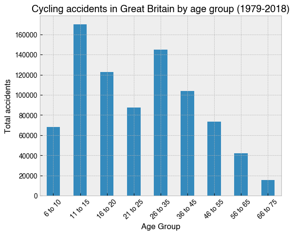
9. Create a bar chart showing how accidents were distributed by Age_Grp

# A list of desired orders for the groups.
# Python's default alphanumeric sorting would place '6 to 10'
# between '56 to 65' and '66 to 75'.
group_order = [
    '6 to 10',
    '11 to 15',
    '16 to 20',
    '21 to 25',
    '26 to 35',
    '36 to 45',
    '46 to 55',
    '56 to 65',
    '66 to 75'
]

# Group by Age_Grp and select the Accident_Index column, which has
# unique values for each accident, making it suitable for a .count() operation
ax = (
    df.groupby('Age_Grp')['Accident_Index']
    .count()[group_order]
    .plot(kind='bar', rot=45)
)
ax.set_title('Cycling accidents in Great Britain by age group (1979-2018)')
ax.set_xlabel('Age Group')
ax.set_ylabel('Total accidents');

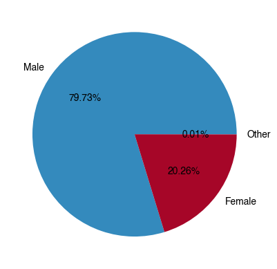
10. Across all accidents, what percentage involved Males, what percentage involved Females, and what percentage involved people identifying as ‘Other’? Show the results in a pie chart.

ax = (
    df.Gender.value_counts()
    .plot
    .pie(autopct='%1.2f%%')  # Add percentage text labels
)
ax.set_ylabel('');

11. What was the highest number of vehicles involved in a single accident?

# 13, but it is unclear from the data key what counts as a vehicle
df.Number_of_Vehicles.value_counts()

2     758784
1      41786
3      24955
4       1861
5        343
6         72
7         30
8         21
9          4
10         3
12         1
13         1
Name: Number_of_Vehicles, dtype: int64

12. What was the highest number of casualties involved in a single accident?

# 60
df.Number_of_Casualties.value_counts().sort_index()

1     792685
2      32367
3       2227
4        357
5        123
6         54
7         23
8          9
9          5
10         3
12         1
13         5
34         1
60         1
Name: Number_of_Casualties, dtype: int64

13. On which day of the week did the accident with Accident_Index 201443N027074 occur?

# Saturday
df.loc[df.Accident_Index=='201443N027074']

	Accident_Index	Number_of_Vehicles	Number_of_Casualties	Date	Time	Speed_limit	Road_conditions	Weather_conditions	Day	Road_type	Light_conditions	Gender	Severity	Age_Grp
751599	201443N027074	2	1	2014-05-07	19:30	30.0	Dry	Clear	Saturday	Single carriageway	Daylight	Male	Serious	16 to 20

# Just get the day
df.loc[df.Accident_Index=='201443N027074'].Day

751599    Saturday
Name: Day, dtype: object

14. Create a separate DataFrame for all serious accidents that happened on a Sunday in wet road conditions. How many were there?

# Create new DataFrame
df2 = df.loc[(
    (df.Severity=='Serious')
    & (df.Day=='Sunday')
    & (df.Road_conditions=='Wet')
)]
df2

	Accident_Index	Number_of_Vehicles	Number_of_Casualties	Date	Time	Speed_limit	Road_conditions	Weather_conditions	Day	Road_type	Light_conditions	Gender	Severity	Age_Grp
9	197901A7PDD49	2	1	1979-07-01	15:15	30.0	Wet	Rain	Sunday	Unknown	Daylight	Male	Serious	11 to 15
107	197901ALMAE81	2	1	1979-01-21	12:00	30.0	Wet	Fog	Sunday	Single carriageway	Daylight	Male	Serious	56 to 65
657	197901D8LGF35	2	1	1979-08-04	11:30	30.0	Wet	Rain	Sunday	Single carriageway	Daylight	Male	Serious	6 to 10
1538	197901FOJEV59	2	1	1979-06-24	09:20	30.0	Wet	Rain	Sunday	Unknown	Daylight	Male	Serious	46 to 55
1542	197901FOPGC24	2	1	1979-06-24	15:30	30.0	Wet	Unknown	Sunday	Unknown	Daylight	Male	Serious	16 to 20
...	...	...	...	...	...	...	...	...	...	...	...	...	...	...
826325	2018521902418	2	1	2018-02-12	16:56	20.0	Wet	Rain	Sunday	Single carriageway	Darkness lights lit	Male	Serious	26 to 35
826477	2018530806661	2	1	2018-07-29	18:50	30.0	Wet	Rain	Sunday	Single carriageway	Daylight	Male	Serious	46 to 55
827229	201863C114718	2	1	2018-09-30	15:35	30.0	Wet	Clear	Sunday	Single carriageway	Daylight	Male	Serious	46 to 55
827580	2018961800246	2	1	2018-07-15	11:00	60.0	Wet	Rain	Sunday	Single carriageway	Daylight	Female	Serious	56 to 65
827618	201897GC01011	3	1	2018-11-25	10:30	60.0	Wet	Clear	Sunday	Single carriageway	Daylight	Male	Serious	56 to 65

2621 rows × 14 columns

# Get the number of entries
len(df2)

2621

15. Create and assign a new `DatetimeIndex <https://pandas.pydata.org/pandas-docs/stable/reference/api/pandas.DatetimeIndex.html>`__ for the DataFrame using the Date and Time columns

# Concatenate Date and Time columns to make datetime-like string
# and convert to DateTimeIndex
df.index = pd.DatetimeIndex(df.Date + ' ' + df.Time)
df

	Accident_Index	Number_of_Vehicles	Number_of_Casualties	Date	Time	Speed_limit	Road_conditions	Weather_conditions	Day	Road_type	Light_conditions	Gender	Severity	Age_Grp
1979-01-01 18:20:00	197901A1SEE71	2	1	1979-01-01	18:20	50.0	Snow	Unknown	Monday	Dual carriageway	Darkness lights lit	Male	Serious	36 to 45
1979-02-01 09:15:00	197901A2JDW40	1	1	1979-02-01	09:15	30.0	Snow	Unknown	Tuesday	Unknown	Daylight	Male	Slight	46 to 55
1979-04-01 08:45:00	197901A4IJV90	2	1	1979-04-01	08:45	30.0	Snow	Unknown	Thursday	Unknown	Daylight	Male	Slight	46 to 55
1979-04-01 13:40:00	197901A4NIE33	2	1	1979-04-01	13:40	30.0	Wet	Unknown	Thursday	Unknown	Daylight	Male	Slight	36 to 45
1979-04-01 18:50:00	197901A4SKO47	2	1	1979-04-01	18:50	30.0	Wet	Unknown	Thursday	Unknown	Darkness lights lit	Male	Slight	46 to 55
...	...	...	...	...	...	...	...	...	...	...	...	...	...	...
2018-02-07 14:55:00	2018983118818	2	1	2018-02-07	14:55	30.0	Dry	Clear	Monday	Single carriageway	Daylight	Male	Slight	6 to 10
2018-07-24 07:45:00	2018983119218	2	1	2018-07-24	07:45	30.0	Dry	Clear	Tuesday	Single carriageway	Daylight	Male	Serious	56 to 65
2018-10-08 13:25:00	2018983120618	2	1	2018-10-08	13:25	20.0	Dry	Clear	Friday	Single carriageway	Daylight	Male	Serious	11 to 15
2018-07-18 21:10:00	2018983121918	2	1	2018-07-18	21:10	30.0	Dry	Clear	Wednesday	Single carriageway	Daylight	Male	Serious	46 to 55
2018-12-20 15:14:00	2018983133818	2	1	2018-12-20	15:14	30.0	Wet	Rain	Thursday	Single carriageway	Daylight	Male	Serious	6 to 10

827861 rows × 14 columns

16. Add a new column to the DataFrame called long_date. It should contain the correct dates matching the following format.

• Wednesday 09 February 2012

# Use date formatting codes
df['long_date'] = df.index.strftime('%A %d %B %Y')
df

	Accident_Index	Number_of_Vehicles	Number_of_Casualties	Date	Time	Speed_limit	Road_conditions	Weather_conditions	Day	Road_type	Light_conditions	Gender	Severity	Age_Grp	long_date
1979-01-01 18:20:00	197901A1SEE71	2	1	1979-01-01	18:20	50.0	Snow	Unknown	Monday	Dual carriageway	Darkness lights lit	Male	Serious	36 to 45	Monday 01 January 1979
1979-02-01 09:15:00	197901A2JDW40	1	1	1979-02-01	09:15	30.0	Snow	Unknown	Tuesday	Unknown	Daylight	Male	Slight	46 to 55	Thursday 01 February 1979
1979-04-01 08:45:00	197901A4IJV90	2	1	1979-04-01	08:45	30.0	Snow	Unknown	Thursday	Unknown	Daylight	Male	Slight	46 to 55	Sunday 01 April 1979
1979-04-01 13:40:00	197901A4NIE33	2	1	1979-04-01	13:40	30.0	Wet	Unknown	Thursday	Unknown	Daylight	Male	Slight	36 to 45	Sunday 01 April 1979
1979-04-01 18:50:00	197901A4SKO47	2	1	1979-04-01	18:50	30.0	Wet	Unknown	Thursday	Unknown	Darkness lights lit	Male	Slight	46 to 55	Sunday 01 April 1979
...	...	...	...	...	...	...	...	...	...	...	...	...	...	...	...
2018-02-07 14:55:00	2018983118818	2	1	2018-02-07	14:55	30.0	Dry	Clear	Monday	Single carriageway	Daylight	Male	Slight	6 to 10	Wednesday 07 February 2018
2018-07-24 07:45:00	2018983119218	2	1	2018-07-24	07:45	30.0	Dry	Clear	Tuesday	Single carriageway	Daylight	Male	Serious	56 to 65	Tuesday 24 July 2018
2018-10-08 13:25:00	2018983120618	2	1	2018-10-08	13:25	20.0	Dry	Clear	Friday	Single carriageway	Daylight	Male	Serious	11 to 15	Monday 08 October 2018
2018-07-18 21:10:00	2018983121918	2	1	2018-07-18	21:10	30.0	Dry	Clear	Wednesday	Single carriageway	Daylight	Male	Serious	46 to 55	Wednesday 18 July 2018
2018-12-20 15:14:00	2018983133818	2	1	2018-12-20	15:14	30.0	Wet	Rain	Thursday	Single carriageway	Daylight	Male	Serious	6 to 10	Thursday 20 December 2018

827861 rows × 15 columns

Read more about date formatting codes

17. What is the worst day on record in terms of the number of accidents that were reported?

# 1983-11-25
df.groupby(df.index.date)['Accident_Index'].count().sort_values()

2010-12-25      2
2009-01-01      2
2017-10-12      3
2003-01-01      3
2007-12-25      3
             ...
1984-07-23    152
1983-07-21    154
1983-07-25    154
1989-07-26    161
1983-11-25    166
Name: Accident_Index, Length: 14609, dtype: int64

# Get the long format date
df.groupby(df.long_date)['Accident_Index'].count().sort_values().index[-1]

'Friday 25 November 1983'

18. Make a bar chart showing total accidents by month of the year

months = ['Jan', 'Feb', 'Mar', 'Apr', 'May', 'Jun', 'Jul', 'Aug', 'Sep', 'Oct', 'Nov', 'Dec']
ax = (
    df.groupby(df.index.month)['Accident_Index']
    .count()
    .plot(kind='bar')
)
ax.set_xticklabels(months, rotation=45)
ax.set_ylabel('Total accidents')
ax.set_title('Cycling accidents by month in Great Britain (1979-2018)');

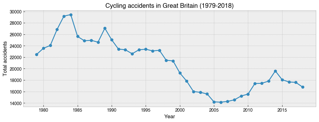
19. Make a line graph showing the total number of accidents that occurred each year from 1979-2018. Have accidents declined overall? In which years did the most and least cycling accidents occur?

# 1984, 2006
ax = (
    df.groupby(df.index.year)['Accident_Index']
    .count()
    .plot(kind='line', marker='o', figsize=(12, 4))
)
ax.set_ylabel('Total accidents')
ax.set_xlabel('Year')
ax.set_title('Cycling accidents in Great Britain (1979-2018)');

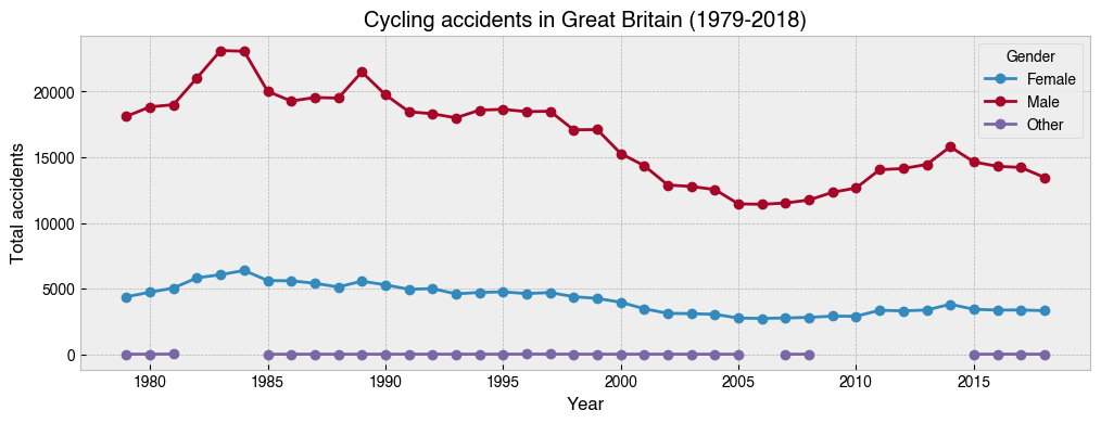
20. Repeat the above, but this time with separate lines for ``Gender``

ax = (
    df.groupby([df.index.year, 'Gender'])['Accident_Index']  # Add Gender to the groupby
    .count()
    .unstack()
    .plot(kind='line', marker='o', figsize=(12, 4))
)
ax.set_ylabel('Total accidents')
ax.set_xlabel('Year')
ax.set_title('Cycling accidents in Great Britain (1979-2018)');

21. Repeat the above, but this time with separate lines for ``Age_Grp``

group_order = [
    '6 to 10',
    '11 to 15',
    '16 to 20',
    '21 to 25',
    '26 to 35',
    '36 to 45',
    '46 to 55',
    '56 to 65',
    '66 to 75'
]
ax = (
    df.groupby([df.index.year, 'Age_Grp'])['Accident_Index']  # Add Age_Grp to the groupby
    .count()
    .unstack()[group_order]
    .plot(kind='line', marker='o', figsize=(12, 4))
)
ax.set_ylabel('Total accidents')
ax.set_title('Cycling accidents in Great Britain (1979-2018)')
ax.legend(title='Age group');

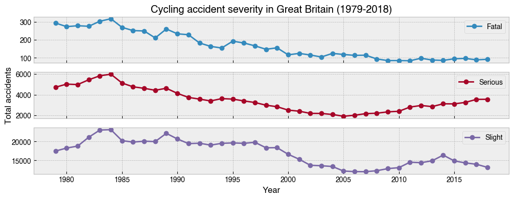
22. Repeat the above, but this time with separate subplots for ``Severity``

axs = (
    df.groupby([df.index.year, 'Severity'])['Accident_Index']  # Add Severity to the groupby
    .count()
    .unstack()
    .plot(kind='line', marker='o', figsize=(12, 4), subplots=True)
)
axs[1].set_ylabel('Total accidents')
axs[2].set_xlabel('Year')
axs[0].set_title('Cycling accident severity in Great Britain (1979-2018)');

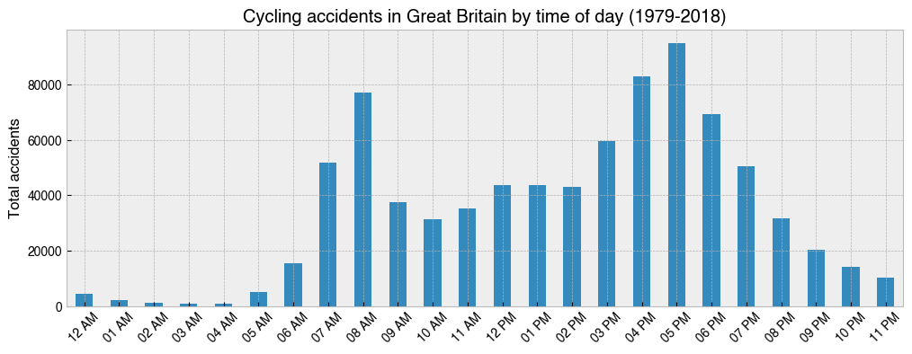
23. Make a bar chart showing the total number of accidents for each hour in the day from 1979-2018

import datetime

ax = (
    df.groupby(df.index.hour)['Accident_Index']
    .count()
    .plot(kind='bar', figsize=(12, 4))
)
ax.set_ylabel('Total accidents')
ax.set_title('Cycling accidents in Great Britain by time of day (1979-2018)')
hours = [datetime.time(i).strftime('%I %p') for i in range(24)]  # Create xticklabels
ax.set_xticklabels(hours, rotation=45);

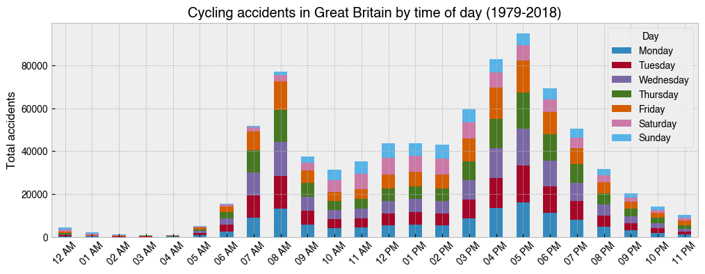
24. As above, but with stacked bars using different colours for each day of the week

import datetime

group_order = ['Monday', 'Tuesday', 'Wednesday', 'Thursday', 'Friday', 'Saturday', 'Sunday']

ax = (
    df.groupby([df.index.hour, 'Day'])['Accident_Index']
    .count()
    .unstack()[group_order]
    .plot(kind='bar', figsize=(12, 4), stacked=True)  # Use stacked option
)
ax.set_ylabel('Total accidents')
ax.set_title('Cycling accidents in Great Britain by time of day (1979-2018)')
hours = [datetime.time(i).strftime('%I %p') for i in range(24)]
ax.set_xticklabels(hours, rotation=45);

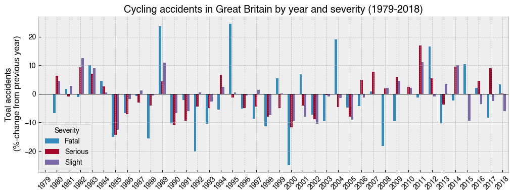
25. Make a bar chart showing the year-on-year percentage change for accidents with different coloured bars for each Severity

ax = (
    df.groupby([df.index.year, 'Severity'])['Accident_Index']
    .count()
    .unstack()
    .pct_change()  # Calculates percentage change from previous value
    .mul(100)  # Times 100 to get percent
    .plot
    .bar(figsize=(12, 4), rot=45, width=.6)
)

ax.axhline(0, 0, 1, lw=.6, c='k')
ax.set_ylabel('Toal accidents\n (%-change from previous year)')
ax.set_title('Cycling accidents in Great Britain by year and severity (1979-2018)');